ts2vg: Time series to visibility graphs#
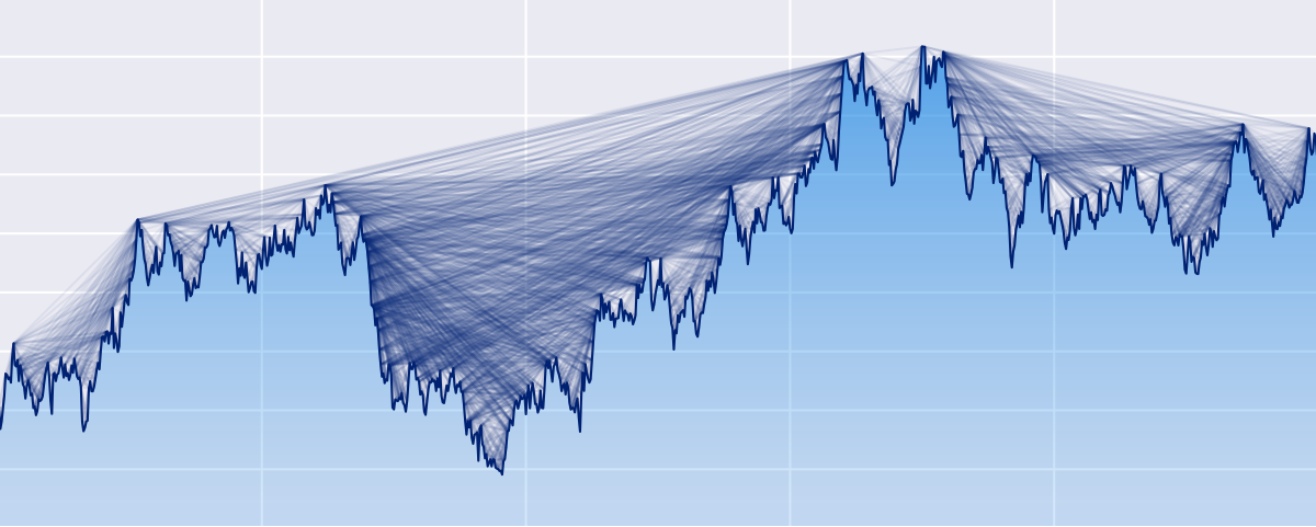
The Python ts2vg package provides high-performance algorithm implementations to build visibility graphs from time series data, as first introduced by Lucas Lacasa et al. in 2008 [1].
The visibility graphs and some of their properties (e.g. degree distributions) are computed quickly and efficiently even for time series with millions of observations. An efficient divide-and-conquer algorithm is used to compute the graphs whenever possible [3].
Installation#
The latest released ts2vg version is available at the Python Package Index (PyPI) and can be easily installed by running:
pip install ts2vg
For other advanced uses, to build ts2vg from source Cython is required.
Supported graph types#
Main graph types#
Available variations#
Additionally, the following variations of the previous main graph types are available:
Weighted Visibility Graphs (via the
weightedparameter)Directed Visibility Graphs (via the
directedparameter)Parametric Visibility Graphs [5] (via the
min_weightandmax_weightparameters)Limited Penetrable Visibility Graphs (LPVG) [4] [6] (via the
penetrable_limitparameter)
Note that multiple graph variations can be combined and used at the same time.
Documentation#
Usage and reference documentation for ts2vg can be found at carlosbergillos.github.io/ts2vg.
Basic usage#
To build a visibility graph from a time series do:
from ts2vg import NaturalVG

ts = [1.0, 0.5, 0.3, 0.7, 1.0, 0.5, 0.3, 0.8]

vg = NaturalVG()
vg.build(ts)

edges = vg.edges
The time series passed (ts) can be any one-dimensional iterable, such as a list or a numpy 1D array.
By default, the input observations are assumed to be equally spaced in time.
Alternatively, a second 1D iterable (xs) can be provided for unevenly spaced time series.
Horizontal visibility graphs can be obtained in a very similar way:
from ts2vg import HorizontalVG

ts = [1.0, 0.5, 0.3, 0.7, 1.0, 0.5, 0.3, 0.8]

vg = HorizontalVG()
vg.build(ts)

edges = vg.edges
If we are only interested in the degree distribution of the visibility graph
we can pass only_degrees=True to the build method.
This will be more efficient in time and memory than storing the whole graph.
vg = NaturalVG()
vg.build(ts, only_degrees=True)

ks, ps = vg.degree_distribution
Directed graphs can be obtained by using the directed parameter
and weighted graphs can be obtained by using the weighted parameter:
vg1 = NaturalVG(directed="left_to_right")
vg1.build(ts)

vg2 = NaturalVG(weighted="distance")
vg2.build(ts)

vg3 = NaturalVG(directed="left_to_right", weighted="distance")
vg3.build(ts)

vg4 = HorizontalVG(directed="left_to_right", weighted="h_distance")
vg4.build(ts)
For more information and options see: Examples and API Reference.
Interoperability with other libraries#
The graphs obtained can be easily converted to graph objects from other common Python graph libraries such as igraph, NetworkX and SNAP for further analysis.
The following methods are provided:
as_igraph()as_networkx()as_snap()
For example:
vg = NaturalVG()
vg.build(ts)

g = vg.as_networkx()
Command line interface#
ts2vg can also be used as a command line program directly from the console:
ts2vg ./timeseries.txt -o out.edg
For more help and a list of options run:
ts2vg --help
Contributing#
ts2vg can be found on GitHub. Pull requests and issue reports are welcome.
License#
ts2vg is licensed under the terms of the MIT License.


